GOALS OF THE PROJECT
The main goal of the Cloud System Evolution in the Trades (CSET) study is to make observations of the stratus-to-cumulus cloud transition occurring along the east and south sides of the Pacific High. By flying trajectories within the north-Pacific trade winds on the NSF/NCAR Gulfstream V (HIAPER), we can follow the evolution of the boundary layer cloud, aerosol, and thermodynamic structures to characterize each regime and understand the transitions between them. The observational data set can also be used in cloud models to simulate the cloud evolution in the trades, a transition that it important to the climate system.
Science Goals:
UM Press Release
Science Goals:
- Define the evolution of the cloud, precipitation and aerosol fields in stratocumulus clouds as they transition into the fair-weather cumulus regimes within the subtropical easterlies over the northern Pacific.
- Examine the cloud microphysical properties and processes as a function of boundary-layer depth, towards assessing the relative contributions of internal and external processes to boundary layer decoupling.
- Assess the relative importance of boundary layer deepening and precipitation processes in driving boundary layer decoupling and cloud breakup.
- Develop integrated data sets and use them to evaluate Large Eddy Simulation (LES) model simulations of cloud system evolution relying on differing resolution and complexities.
UM Press Release
OBSERVATION STRATEGIES
To study the evolution of clouds, we are using a Lagrangian approach, where we target trajectories going across the transition zone and sample them once at the start and again 48 hours later. These trajectories are created using the NOAA HYSPLIT model. A sample set of trajectories can be seen in Figure 11, where the star on each line represents the initial position of the air mass, and the square represents the predicted location of that air mass in 48 hours. Our goal is to chose a few trajectories that start in the stratus or stratocumulus regime, travel generally with the trade winds, and end up in the cumulus regime. We also have to be careful that they don't travel too far or diverge too much to make it difficult to sample the end points of the trajectories 48 hours later. For example, trajectories 28, 27, 21, and 15 in Figure 11 move in the general direction with the trades and move at a reasonable speed. We create a flight plan using some combination of these trajectories or points between them. We then fly from Sacramento, California to Kona, Hawaii going through the selected trajectory starting points (known as waypoints), and return from Hawaii to California 48 hours later through the end points of the chosen trajectories.
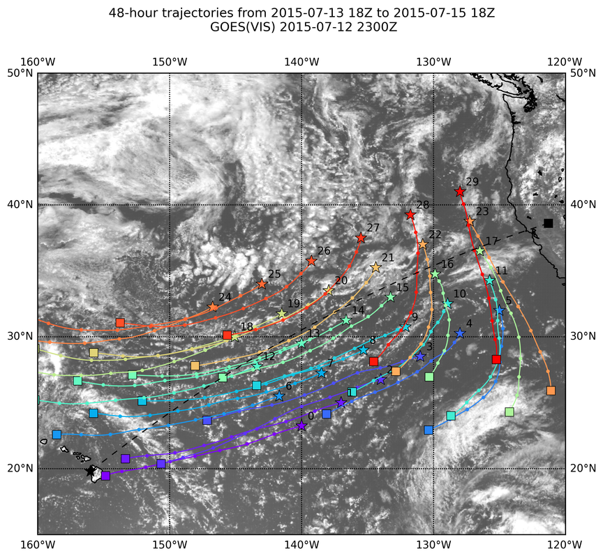
Figure 11: Forecasted sample trajectories for 7/15/15. The stars show the starting location of the air mass (where we would attempt to sample on our outbound flight), and the line shows how that air is forecast to move with time. Each dot in the line represents 6 hours, and the squares show the forecast location of the air at the end of 48 hours (where we would attempt to sample on our return flight). Image from the EOL CSET field catalog model page.
On the flight from California to Hawaii, we ferry out to the waypoints at a height of about 20,000-28,000 feet. At this altitude, we are well positioned for optimal data from the downward viewing radar and lidar. We are also able to launch dropsondes from flight level to the surface every 2° (on even degrees of longitude) to obtain the thermodynamic and wind structure above the boundary layer. Flying at an altitude well above the cloud layer and inversion is known as surveying mode where remote sensing is the dominant method of data collection.
Once we reach the start of the targeted zone where the chosen trajectories begin, we switch to in situ mode, where the plane flies in the boundary layer (BL) following the pattern shown in Figure 12. We begin to descend about 40 minutes before reaching the start of the first trajectory so the plane reaches 500 feet at our first waypoint. During that initial descent, the science team is able to determine the height of the cloud top (either visually, where the coldest temperature in the inversion is found, or where RH drops below 70% above) and cloud base (preferably stratocumulus base). The BL sampling structure* is to fly at 500 feet for 10 minutes as a surface leg, fly at CB+300 ft for 10 minutes for an in cloud leg, "porpoise" up and down 1500 feet in and out of the cloud top (ascent to 1200 ft above CT and descent to 300 ft below cloud top) for 10 minutes, and then fly at CT +3000 ft for 10 minutes for an above cloud leg. One complete BL sample should take about 50 minutes (including time to transition between flight levels). This pattern is then repeated for as many times as necessary to get through the selected waypoints of the trajectory, usually 3-5 cycles depending on time/fuel constraints. A full suite of probes on the aircraft will be used for in situ measurements of aerosol, cloud, precipitation, and turbulence properties.
*Flight patterns in the BL may change at the discretion of the onboard scientists depending on cloud conditions.
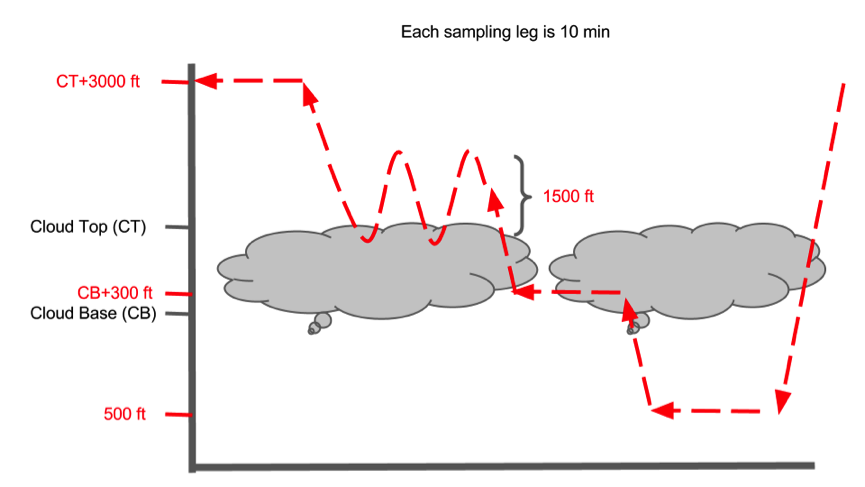
Figure 12: Pattern for in situ sampling of the boundary layer.
After the BL sampling through the waypoints has been completed, the GV increases in altitude back to a ferry height to complete the trip to Hawaii, as seen in Figure 13. During this ferry leg, we return to surveying mode with the radar and lidar and attempt to continue to launch dropsondes every 2° (or every 10-20 minutes) as air traffic allows.
After the BL sampling through the waypoints has been completed, the GV increases in altitude back to a ferry height to complete the trip to Hawaii, as seen in Figure 13. During this ferry leg, we return to surveying mode with the radar and lidar and attempt to continue to launch dropsondes every 2° (or every 10-20 minutes) as air traffic allows.
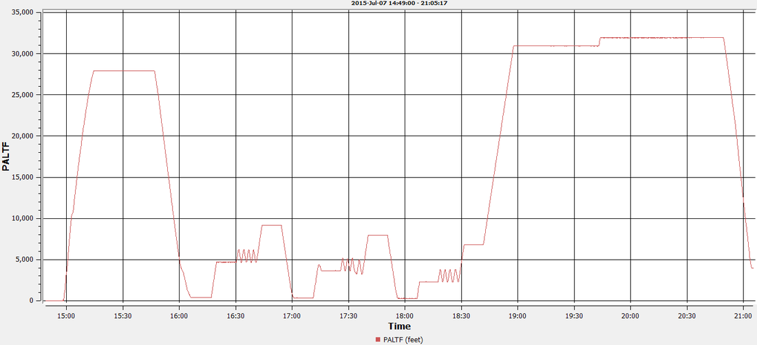
Figure 13: GV altitude with time from RF02 on 7/7/15. The ferry leg out to waypoint 1 can be seen in the first hour (15:00-16:00 UTC), followed by 3 boundary layer sampling patterns similar to Figure 12. Note how the heights of the CB+300 ft and CT+3000 ft legs change with each BL sample. The start of the ferry to complete the flight is shown at 19:00 UTC. The 2nd ferry leg on this flight was above ideal remote sensing heights due to air traffic patterns.
After landing in Hawaii and following a one-day maintenance day, the aircraft returns to CA using the same pattern; with ferry legs to and from the transition zone, and detailed profiling in the sub-cloud and cloud layer along the end points of the selected trajectories. This Lagrangian approach is designed to minimize uncertainties in the large-scale forcing due to horizontal advection in the lower troposphere as air masses move from cold to warm SSTs, and thus facilitate model simulations and isolate critical physical processes.
After one or two down days, another flight cycle is initiated from CA if cloud conditions are favorable. All research flights for CSET can be seen in the EOL Field Catalog Mission Log. The observations made on these flights will be used to evaluate the moisture, dry static energy and mass budgets by estimating the changes in these parameters between the upstream stratocumulus region sampled on one flight and the downstream cumulus region sampled on the subsequent flights.
Flight plans are made the afternoon before each flight based on modeled trajectories, pressure systems, LTS, SSTs, and project flight distance, with a go/no-go decision by the mission scientist(s) 2 hours before takeoff.
MEET THE TEAM
Success in a major field project such as CSET requires a collaboration from team members, including research scientists, instrumentation specialists, project and data managers, and flight crew/maintenance.
Many of our team members participated in interviews describing a particular portion of this project. To see these interviews, please click on the links next to each individual.
Many of our team members participated in interviews describing a particular portion of this project. To see these interviews, please click on the links next to each individual.
Bruce Albrecht: Principal Investigator (PI) from University of Miami, RSMAS
John Allison: Field Catalog. Click here for video interview with John.
Clayton Arendt: AVAPS Technician
Lee Baker: Pilot
Tom Baltzer: RAF SE
Chris Bretherton: Co-Investigator (Co-I) from University of Washington: Click here for video interview with Chris.
Chris Burghart: HCR SE
Teresa Campos: Trace Gas Scientist
Shaunna Donaher: Educational Developer from Emory University
Scott Ellis: HCR Scientist
Jonathan Emmett: HCR Technician
Rich Erickson: HSRL Technician
Virendra Ghate: Co-I from Rutgers and Argonne National Laboratory. Click here for a video interview with Virendra.
Susanne Glienke: HOLODEC Scientist. Click here, here, and here for video interviews with Susanne.
Julie Haggerty: MTP Scientists
Samuel Hall: HARP Scientist
Bill Irwin: RAF Technician
Jorgen Jensen: RAF Scientist (Cloud Physics). Click here for a video interview with Jorgen.
Ed Kosciuch: Trace Gas Technician
Bo LeMay: Pilot
Eric Loew: HCR Tecnician
Lou Lussier: Project Manager
Scott Mcclain: Chief Pilot
Jeremy McGibbon: Graduate Student from University of Washington. Click here for video interview with Jeremy.
Hans Mohrmann: Graduate Student from University of Washington. Click here for a video interview with Hans.
Bruce Morley: HSRL Scientist
Jason Morris: Mechanic
Alison Nugent: NSF PostDoc. Click here for video interview with Alison.
Mike Paxton: Systems Administrator
Andrew Pazmany: GVR Scientist
Nick Potts: AVAPS Engineer
Mike Reeves: RAF Scientist (Aerosols)
Ed Ringleman: Pilot
Pavel Romashkin: Project Manager
Mampi Sarkar: Graduate Student from University of Miami, RSMAS. Click here for video interview with Mampi.
Chris Schwartz: Graduate Student
Jeff Stith: Manager, Research Aviation Facility at NCAR. Click here for a video interview with Jeff.
Aaron Steinbach: Mechanic
Meghan Stell: Trace Gas Scientist
Greg Stossmeister: Field Catalog
Peisang Tsai: HCR Engineer. Click here for video interview with Peisang.
Laura Tudor: AVAPS Technician
Kirk Ullmann: HARP Scientist
Joe VanAndel: HSRL SE
Vivek: HCR Scientist. Click here for a video interview with Vivek.
Cory Wolff: Project Manager. Click here for a video interview with Cory.
Robert Wood: Co-I from University of Washington. Click here for video interview with Rob.
Paquita Zuidema: Co-I from University of Miami, RSMAS. Click here for video interview with Paquita.
INSTRUMENTATION
In addition to the advanced observational technology described below, CSET makes use of recent advances in communications and data streaming to allow scientists on the ground to follow along with the mission as if they are on the plane. Two important features that allow this to occur are the real-time data stream through Aeros and the IRC Chat access with the onboard science team and aircraft. These advances allow the team on the ground to monitor the flight and instrument functions and quickly make any necessary adjustments to improve data collection. The ground team is also able to see selected data streaming as it is being collected, which improves future mission planning and enhances scientific discussions.
Aircraft Instrumentation
NSF/NCAR GV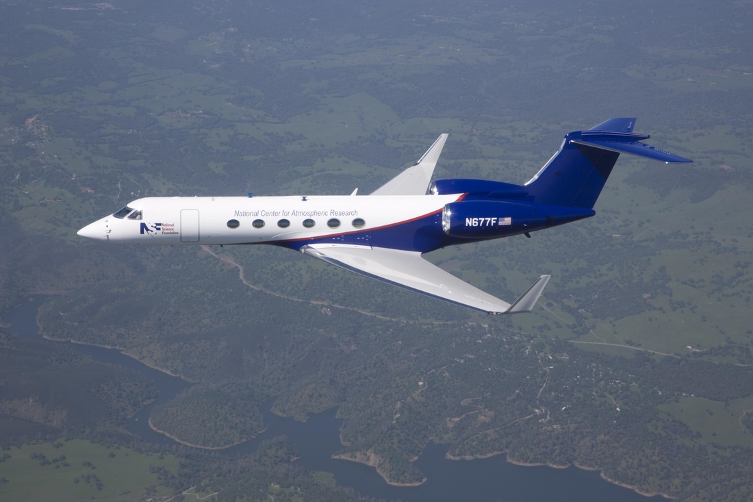
|
The NSF/NCAR Gulfstream-V High-performance Instrumented Airborne Platform for Environmental Research (GV HIAPER) aircraft is a cutting-edge observational platform that has been modified to meet the scientific needs of researchers who study many different aspects of the earth's environment, including projects like CSET which study clouds and aerosols.
The HIAPER is a highly modified Gulfstream V business jet that has unique capabilities that set it apart from other research aircraft. It can reach 51,000 feet (15,500 meters), enabling scientists to collect data from near the earth’s surface to the tops of storms and to the lower edge of the stratosphere. With a range of about 7,000 miles (11,265 kilometers), it can reach many remote locations, allowing for sampling from the North Pole to the South Pole. Payload: https://www.eol.ucar.edu/system/files/CSET_GV_payload.pdf Wing layout: https://www.eol.ucar.edu/system/files/CSET_GV_external_payload.pdf Two key elements of the observing system will be a newly developed HIAPER Cloud Radar (HCR) and the HIAPER Spectral Resolution Lidar (HSRL). The HCR will be used to provide cloud and precipitation characteristics. The HSRL points will provide cloud boundaries and aerosol characteristics when viewing non-cloudy volumes. A full suite of probes on the aircraft will be used for in situ measurements of aerosol, cloud, precipitation, and turbulence properties. |
2DC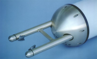
Image from https://www.eol.ucar.edu/node/199
|
Two-Dimensional Optical Array Cloud Probe
Provides two-dimensional images of hydrometeors by recording the two-dimensional shadow cast by a hydrometeor as it passes through a laser beam. |
3V-CPI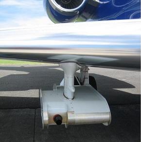
Image of 3v_CPI mounted under a wing on the GV from https://www.eol.ucar.edu/instruments/three-view-cloud-particle-imager
|
Three-View Cloud Particle Imager
Using a combination of 3 imaging instruments, this provides images of hydrometeors, sizes, shapes, and concentrations of hydrometeors with sizes from about 10 um to a few mm. The probe is particularly suited to imaging ice crystals, but also provides good detection of other hydrometeors including large cloud droplets, drizzle and small rain drops, and precipitation particles. This instrument makes ups to 450 photos of ice particles per second. |
AVAPS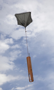
Dropsonde image from https://www2.ucar.edu/atmosnews/in-brief/7188/getting-drop-storms
Dropsondes ready to be launched during RF13. Photo by Chris Bretherton.
|
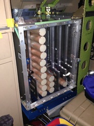
AVAPS Dropsonde System
NCAR Airborne Vertical Atmospheric Profiling System (AVAPS) measures vertical profiles of temperature, pressure, humidity, and wind speed and wind direction (via GPS) as it is launched from the aircraft and descends to the surface. Each sonde takes about 15 minutes to fall to the surface (assuming it is launched from 45,000 ft and has a fall speed of about 11 m/s at the sea surface). Winds are measured every 0.25 seconds, pressure/temperature/humidity are measured every 0.5 seconds. In-situ data collected from the sonde’s sensors are transmitted back in real time to an onboard aircraft data system via radio link. Sondes are 30.5 cm long, 4.7 cm in diameter, weigh 165 grams, and can be launched remotely. An average of 8 sonde launches per flight are planned. Dropsonde History: https://www.eol.ucar.edu/node/176 |
CDP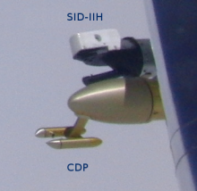
|
Cloud Droplet Probe
The cloud particle distributions are measured with a cloud droplet probe (CDP) by shooting a laser beam into an air sample and detecting light scattered from that beam by cloud droplets. |
CN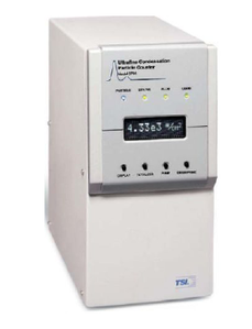
Image from https://www.eol.ucar.edu/node/216
|
Condensation Nucleus Counter (water or butanol)
Condensation nuclei, or particles that act as surfaces for water vapor to condense upon, are detected by exposing a sample of air to supersaturated vapor (either liquid or butanol), and measuring the drops that grow larger than an observable threshold of about 10 nanometers |
COMR_AL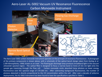
|
Aero-Laser VUV Resonance Fluorescence Carbon Monoxide Instrument
CO concentration is measured using a narrow band of UV light focused on a sample of air. The CO in the air absorbs energy and re-emits it at a particular wavelength, and the intensity of the re-emitted energy can be used to show the concentration of CO in the gas. |
Image from https://www.eol.ucar.edu/node/219
FO3_ACD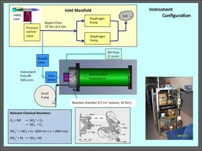
Image from https://www.eol.ucar.edu/node/227
|
Nitric Oxide Chemiluminescence Ozone Instrument
Measures NO in air flowing through the instrument as chemical reactions occur to provide Ozone Mixing Ratio at 1- and 5-Hz. |
GVR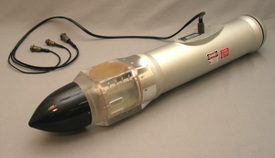
|
G-Band Water Vapor Radiometer
The 183- GHz GVR estimates low concentrations of precipitable water vapor and liquid water path from brightness temperature. |
HARP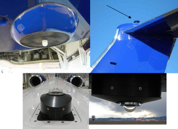
The HARP collectors. Clockwise from upper left: actinic flux, nadir; actinic flux, zenith; irradiance, nadir; irradiance zenith. Image from https://www.eol.ucar.edu/node/228
|
HIAPER Airborne Radiation Package
Uses hemispheric light collectors (similar to sky imagers) looking up and down to measure the amount and intensity of light at certain wavelengths, which can initiate photochemical processes in the atmosphere. |
HCR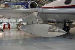
Image from https://www.eol.ucar.edu/node/205
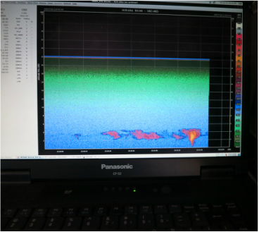
Streaming HCR data onboard RF05. Photo by Bruce Albrecht.
|
HIAPER Cloud Radar
The HCR is a 95 GHz Doppler (W-band) cloud radar developed for HIAPER that characterizes cloud structure via reflectivity and air motion via Doppler velocity. A special wing pod has been developed for the HCR that allows it to point upwards or downwards as needed, allowing for observations of clouds in the boundary layer no matter what level the GV is flying at. In "surveying mode", the cloud radar will be used to remotely provide characteristics of cloud below the flight level, including cloud top height. During the in situ part of the flights, the Doppler capability of the radar will provide the possibility of studying vertical draft structures and turbulence in the clouds. W-band radars are ideal cloud radars because they are sensitive enough to see stratus, stratocumulus, and cumulus clouds, as well as light precipitation. However, the beam may saturate in very thick clouds or moderate precipitation. During non-precipitating conditions (reflectivity < -15 dBZ) the cloud droplets have negligible fall velocities, so the measured Doppler velocity corrected for the aircraft motion can be used as a proxy for the vertical air motion. During precipitating conditions, the fall velocity of precipitating drops must be removed from the measured Doppler velocity to retrieve the vertical air motion. The HCR has a temporal resolution of ~1 second, which gives a horizontal resolution of 100-200 m and range resolution of 40-50 m, with a maximum range of 7.5 km. |
HOLODEC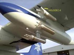
|
Holographic Detector for Clouds
Measures droplet sizes and drop size distribution via a laser holographic technique. This helps to see two-dimensional shapes drops larger than 6 micrometers and three-dimensional positions, which calculates the distance between drops. |
HSRL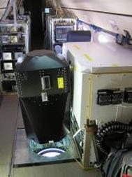
Image from https://www.eol.ucar.edu/node/226
|
High Spectral Resolution Lidar
The HSRL uses a transmitted beam to remotely provide estimates of cloud base and top heights, aerosols, and optically-thin (boundary layer and cirrus) cloud vertical profiles. It also derives estimates of cloud optical depth, aerosol optical depth, scattering cross-section, and extinction cross-section from the profiles of backscatter cross-section. The range resolution of the retrieved backscatter cross-section profiles is ~30 m while that of extinction profile is ~300 m. Like the HCR, the HSRL will be operated looking downwards except during the BL profiling where the plane is flying in the subcloud layer. This method allows for the best observations of cloud structure, cloud tops, cloud bases, and drizzle. |
MTP
Image from https://www.eol.ucar.edu/node/181
|
Microwave Temperature Profiler
The MTP is an airborne passive microwave sounding device that observes emitted radiance (brightness temperature) between 56-59 GHz over a range of scanning angles. It collects measurements of thermal emission from oxygen molecules and converts them into temperature. Acting as a remote sensing instrument, it can measure temperature profiles away from the aircraft at vertical resolutions ranging from 150 m to 1 km. |
UHSAS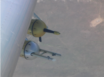
|
Ultra-High Sensitivity Aerosol Spectrometer
The UHSAS measures the concentration and size distribution of aerosol particles having diameters from 0.06-1.0 µm, and categorizes them into size bins. The instrument flies in an under-wing canister and senses particles in the airstream via light scattering from individual particles. |
Satellite Instrumentation
Satellite observations will be used to define the larger-scale (> 100 km x100 km) cloud fields along the aircraft flight path, including cloud cover, cloud liquid water path, sea surface temperature, precipitation, aerosol amount and type, cloud droplet number concentration, and surface winds.
COSMIC Soundings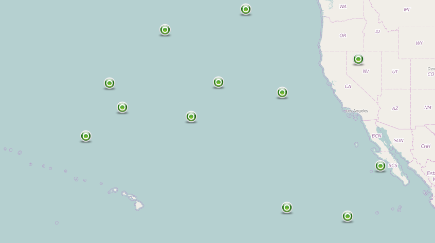
These automated satellite soundings estimate thermodynamic structure in the region. Each green dot in the figure to the left represents the location of a COSMIC Sounding. Image from http://catalog.eol.ucar.edu/cset
|
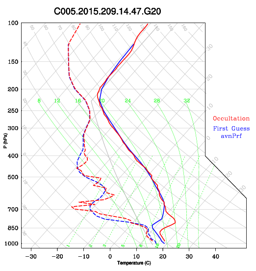
A sample Skew-T diagram with data from a COSMIC sounding on 7/28/2015. Image from http://catalog.eol.ucar.edu/maps/cset
|
VIDEOS FROM THE FIELD
Video of the GV and instrument onboard for the CSET project: https://youtu.be/oEVRs2og-7M
Video of preparations 45 minutes preflight: https://youtu.be/PsDr1kbHDQQ
Video of cockpit 30 minutes preflight: https://youtu.be/tuWLZl1Lx28
Video of clouds during RF04: https://youtu.be/DRzZ3v5gPxI
Video in-flight (1): https://youtu.be/J-3vTZpgRlY
Video in-flight (2): https://youtu.be/Z3EOp7zaj8w
Video of HSRL in-flight: https://youtu.be/obhX_-LI_7Y
Video of HCR in-flight: https://youtu.be/J-ESf99Yc4s
Video of high cloud masking seen using the CSET maps function during a planning meeting: https://youtu.be/eAzzb415ELM
|
|
|
|
|
|
|
|
|
|
|
|
Two animations of trajectories and corresponding satellite images (both created by Mampi Sarkar):
In these videos, the red line denotes the CA to HI flight path; the magenta line shows HI to CA path; yellow stars denote the parcel position every 5 hours; blue star denotes the current position of the parcel; black line denotes the current trajectories; and the blue line denotes previous trajectories.
1) Animation following a trajectory of an air mass sampled in RF06 and RF 07. Notice the clear center of the Pacific High.
2) Animation showing 13 trajectories of air sampled during RF06 and where they end up and are sampled in RF07. This animation zooms in on each of the trajectories to show the cloud transition in greater details.
Other videos (both created by Hans Mohrmann):
Following trajectories between RF06 and RF07: http://www.atmos.washington.edu/~jkcm/CSET_plots/GOES_loops/rf06_rf07_06fps_boxes.mp4
A very cool sped up video of the forward looking camera on the G-V during RF07:
http://www.atmos.washington.edu/~jkcm/CSET_plots/HIAPER_camera/RF07_crf30.mp4
